• Midterm Grades

• Recap:

  • defining of confounding
  • why confounding happens
  • causal graphs

• Recognizing Confounding

  • which additional variables generate confounding?
  • what is the direction of bias

“BC’s face-mask mandate reduced COVID mortality in the province over the course of the pandemic.”

• Fundamental Problem of Causal Inference means we can’t observe BC in the counter-factual world without face-masks.

Karaivanov et al (2020), economists at SFU, investigate:

Did indoor mask mandates reduced COVID cases, on average? If masks reduce COVID cases, could reduce mortality.

They compare COVID cases in Ontario Public Health Units (PHU) with and without mask mandates

• Not all Ontario PHUs imposed mask mandates at the same time
• Can compare PHUs with and without mandates
• Correlation of mask mandates and COVID cases across PHUs

They find that PHUs with mask mandates have slower COVID case growth than PHUs without mask mandates…

• Is there any reason to doubt that this is the causal effect of mask mandates?

Correlation suffers from two sources of error:

random error: we observe patterns in \(X\) (independent variable) and \(Y\) (dependent variable) by chance, when there is in fact no relationship.

confounding (bias): the systematic observed pattern between \(X\) and \(Y\) is not the true causal relationship between \(X\) and \(Y\).

confounding is when there is a systematic observed correlation between \(X\) and \(Y\) that does NOT reflect the true causal effect of \(X\) on \(Y\).

• This is not a chance correlation.
• Two ways to explain why this happens (different explanations, but two sides of the same coin)

It’s summer of 2020… the correlation Karaivanov et al use effectively compares…

COVID caseload in PHUs in Toronto area (with mask mandates)…

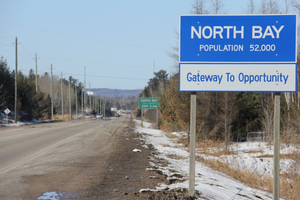
… with COVID caseload in PHUs like North Bay (without a mask mandate)

Correlation means we “plug in” missing counterfactuals from other cases:

If this equivalence \((=)\) is false, then confounding (bias)

Why Confounding?

Confounding occurs because:

We use outcome in case B (North Bay) to stand in for counterfactual outcome from case A (Toronto). But outcomes in case B are not the same as in counterfactual case A.

Two ways of thinking about why this produces a bias; unifying idea is that case A and B are different in ways other than X. These other differences affect X and Y.

Confounding and Causal Graphs

Explanation 1: visual

Confounding occurs when these other differences between cases (third variables, e.g. \(W\)) causally affect \(X\) and \(Y\).

This can be seen visually

Causal graphs represent a model of the true causal relationships between variables.

the nodes or dots correspond to variables

• can be labeled with generic names for independent/dependent variables (\(X\), \(Y\)) or meaningful names (e.g. “Mask Mandate”, “COVID Cases”)

the arrows convey the direction of causality

• \(X \rightarrow Y\) means that \(X\) causes changes in \(Y\)
• \(X \leftarrow W\) means that \(W\) causes changes in \(X\)

A model of true causal relationships, because:

• we don’t know the true causal relationships for sure
• graphs permit us to think whether there is confounding, assuming a particular story about what causes what

For example

PHUs in Toronto (that had a mask mandate) may have a larger population of university educated adults than PHUs in North Bay (no mask mandate).

• University educated residents might be more likely to work from home \(\xrightarrow{causes}\) mask mandate affects fewer people \(\xrightarrow{causes}\) more likely to mandate masks
• University educated residents \(\xrightarrow{causes}\) work from home \(\xrightarrow{causes}\) fewer social contacts \(\xrightarrow{causes}\) lower COVID cases

In a causal graph, there is confounding of correlation of \(X\) and \(Y\) if…

1. some other variable \(W\) has causal paths toward \(X\) and \(Y\)
2. (equivalently) there is backdoor path or non-causal path from \(X\) to \(Y\)
   • a chain of two or more arrows that follows arrows backwards out of \(X\), changes direction once and follows arrows toward \(Y\): \(X \leftarrow W \leftarrow Z \rightarrow Y\)

Confounding?

Why do backdoor paths produce confounding? Why is it systematic?

Explanation 2: Other differences, Different potential outcomes

• antecedent variables
  • sometimes confounding
  • sometimes no confounding
• intervening variables
  • no confounding
• reverse causality
  • yes, confounding.

antecedent variable: a variable that affects \(X\)

• e.g. in this path, \(W \xrightarrow{} X \xrightarrow{} Y\), \(W\) is an antecedent variable.

• antecedent variables (\(W\)) do not produce confounding if the only causal path from \(W\) to \(Y\) passes through \(X\).

• antecedent variables do produce confounding if there is another causal path from \(W\) to \(Y\) that does NOT include \(X\).

• No. No “backdoor” path.

• No. No “backdoor” path.

• Yes. Mandate \(\xleftarrow{}\) Positives \(\xrightarrow{}\)Stay Home\(\xrightarrow{}\)COVID Cases

• No. No “backdoor” path; apparent “backdoor” changes directions more than once.

intervening variable: a variable that affects \(Y\) and is affected by \(X\).

• e.g. in this path, \(X \xrightarrow{} M \xrightarrow{} Y\), \(M\) is an intervening variable.

• intervening variables (\(M\)) do not produce confounding because they are on the causal path from \(X\) to \(Y\). They do not produce backdoor path.

• No backdoor path. Mask mandate affects COVID through mask wearing.

• No backdoor path. Mask mandate affects COVID through mask wearing, avoiding indoor spaces.

reverse causality describes the situation where the dependent variable \(Y\) actually causes the independent variable \(X\).

So while we use the correlation to describe the effect of \(X\) on \(Y\): \(X \to Y\), the correlation in fact is the result of the effect of \(Y\) on \(X\): \(Y \to X\).

This is a special case of bias or confounding.

Gun violence in Miami Beach has led to state of emergency and curfew during Spring Break.

“We haven’t been able to figure out how to stop spring break from coming,” Mr. Gelber said. “We don’t want spring break here, but they keep coming.”

Does reducing the number of guns reduce firearms violence (deaths)?

• Correlation of gun ownership and gun deaths for US states.

Does gun ownership slightly reduce firearms deaths?

Let’s say Miami Beach is considering imposing gun control policies to reduce gun deaths during Spring Break. To make their decision, they look at the correlation on the previous slide…

If that correlation suffered from confounding (bias), how might it affect the policy decision and its consequences…

• if the confounding induced an upward bias (correlation between gun ownership and firearms deaths more positive than true causal relationship)?
• if the confounding induced a downward bias (correlation between gun ownership and firearms deaths more negative than true causal relationship)?

Why do we care?

As with measurement bias, we need to apply weak severity principle to judge whether bias would present a problem.

• If bias is upward and correlation is negative, true causal effect is MORE negative. \(\to\) Definitely don’t use gun control

• If bias is downward and correlation is negative, true causal effect direction is unknown. \(\to\) Unclear what policy to choose. (Fails weak severity — confounding leads us to find negative causal effect even if truth is positive causal effect)

Product of signs on causal path from \(W \to X\) and \(W \to Y\) gives us direction of bias created by confounding

\(^*:\) this only works for a single backdoor paths; not the total of multiple backdoor paths. Then we would need more information.

We now know what confounding is and how it arises…

Consider the case of gun-control laws and gun violence::

• is there any way we set up a correlation where we can guarantee no other variable \(W\) affects \(X\) (cause) and \(Y\) (outcome)? If yes, what is it?

Causal graphs point us to possible solutions:

If something else (\(W\)) changes \(X\) and \(Y\), leading to confounding…

1. We can use comparisons that hold \(W\) constant.

   • but do we know all relevant differences? (all causal paths?)

2. We can use comparisons that break the connection between \(W\) and \(X\).

   • how do we break this connection?

Confounding

1. bias: observed correlation \(\neq\) true casual relationship
2. Why?
   • cases with different values of \(X\), also differ in \(\text{factual}, \color{red}{\text{counterfactual}}\) values of \(Y\)
   • when “third” variable affects \(X\), affects \(Y\) \(\to\) confounding.
3. Causal graphs help us diagnose possible sources of confounding.
4. Causal graphs help us diagnose the expected direction of bias

• Causal graphs also point to possible solutions for confounding